How you can Import Information from One Google Sheet to One other

Having your information unfold out throughout totally different spreadsheets is a typical problem. You might need gross sales figures in a single file, stock information in one other, and buyer info in a 3rd sheet. When it is advisable to pull that info collectively to construct a dashboard or a abstract report, the default answer is commonly guide copying and pasting.

What in case your Google Sheets might speak to one another, routinely updating your reviews at any time when the supply information modifications?

On this information, we’ll discover all of the highly effective methods to import information between totally different Google Sheets.

Additionally see: Create Inventory Dashboard in Google Sheets

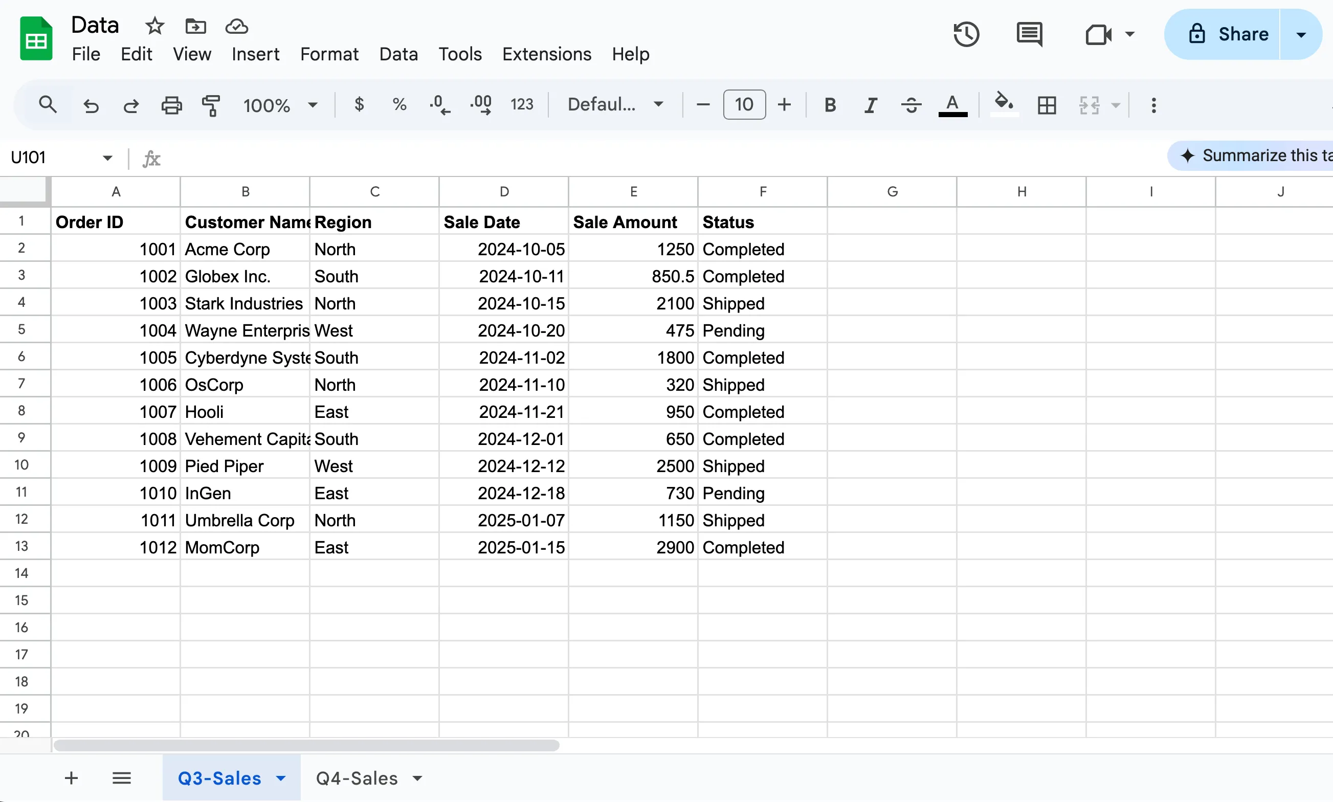
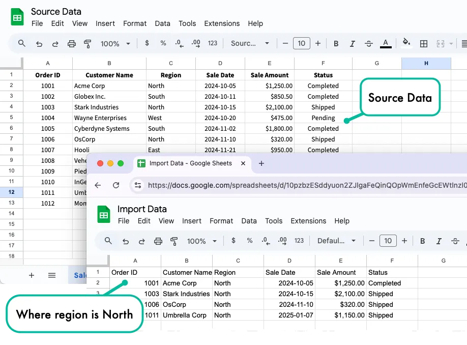
For our examples, we’ll use a supply Google Spreadsheet with a sheet named Gross sales. This sheet comprises buyer names, areas, gross sales quantities, and different particulars that we’ll be importing into different Google Sheets.

#1. Import Information with IMPORTRANGE

The IMPORTRANGE perform in Google Sheets permits you to herald information from a wholly totally different spreadsheet, sustaining a reside connection between the supply and vacation spot. This reside hyperlink ensures that your reviews and dashboards at all times replicate essentially the most up-to-date info, with no need to manually copy or replace information.

The one requirement for IMPORTRANGE is that the supply spreadsheet have to be accessible to the particular person importing the info. For those who’re importing from a sheet you don’t personal, make sure the proprietor has granted you editor or viewer entry.

To make use of the IMPORTRANGE perform, it is advisable to present the URL of the supply spreadsheet and the vary of cells you wish to import. For instance, if you wish to import the info from the Gross sales sheet, the vary can be one thing like Gross sales!A1:F50. If the sheet identify comprises areas, it is advisable to wrap it in single quotes like 'Q3 Gross sales'!A1:F50.

The syntax for the IMPORTRANGE perform is easy:

=IMPORTRANGE(spreadsheet_url, range_string)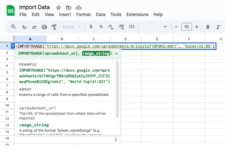

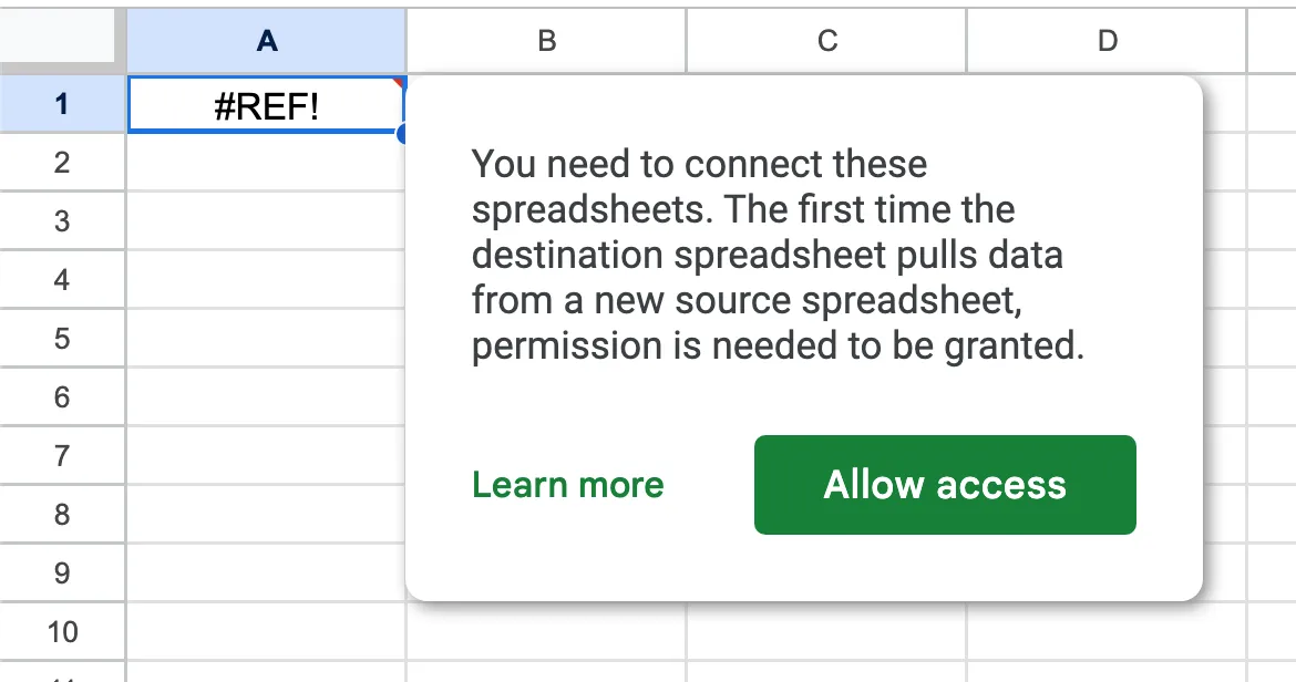
The primary time you add this perform to your spreadsheet cell, it can return a #REF! error. This merely means Google Sheets wants your permission to entry the supply spreadsheet. Hover your mouse over the error and click on on Enable entry to grant entry. This authorization is remembered, so that you solely must do it as soon as per vacation spot spreadsheet.

Going again to our earlier instance, if we want to import the header row and the primary 12 rows of information from the Gross sales sheet into a brand new sheet, our system would appear to be this:

=IMPORTRANGE("https://docs.google.com/spreadsheets/d/1234567890/edit", "Gross sales!A1:F13")

#2. Mix A number of Ranges with IMPORTRANGE

The ability of IMPORTRANGE isn’t restricted to pulling a single vary. You may mix information from a number of ranges -even from totally different sheets or spreadsheets – into one steady listing utilizing array literals {}.

The array syntax {} tells Google Sheets to construct a customized array, or listing, of information based mostly in your directions. There are two main methods to rearrange your mixed information:

2.1. Vertical Stacking (Place information one on high of the opposite)

That is the commonest and highly effective method to mix information. By separating your IMPORTRANGE formulation with a semicolon;, you’ll be able to merge information from totally different sheets (and even totally different spreadsheets) right into a single listing the place the info is positioned one on high of the opposite.

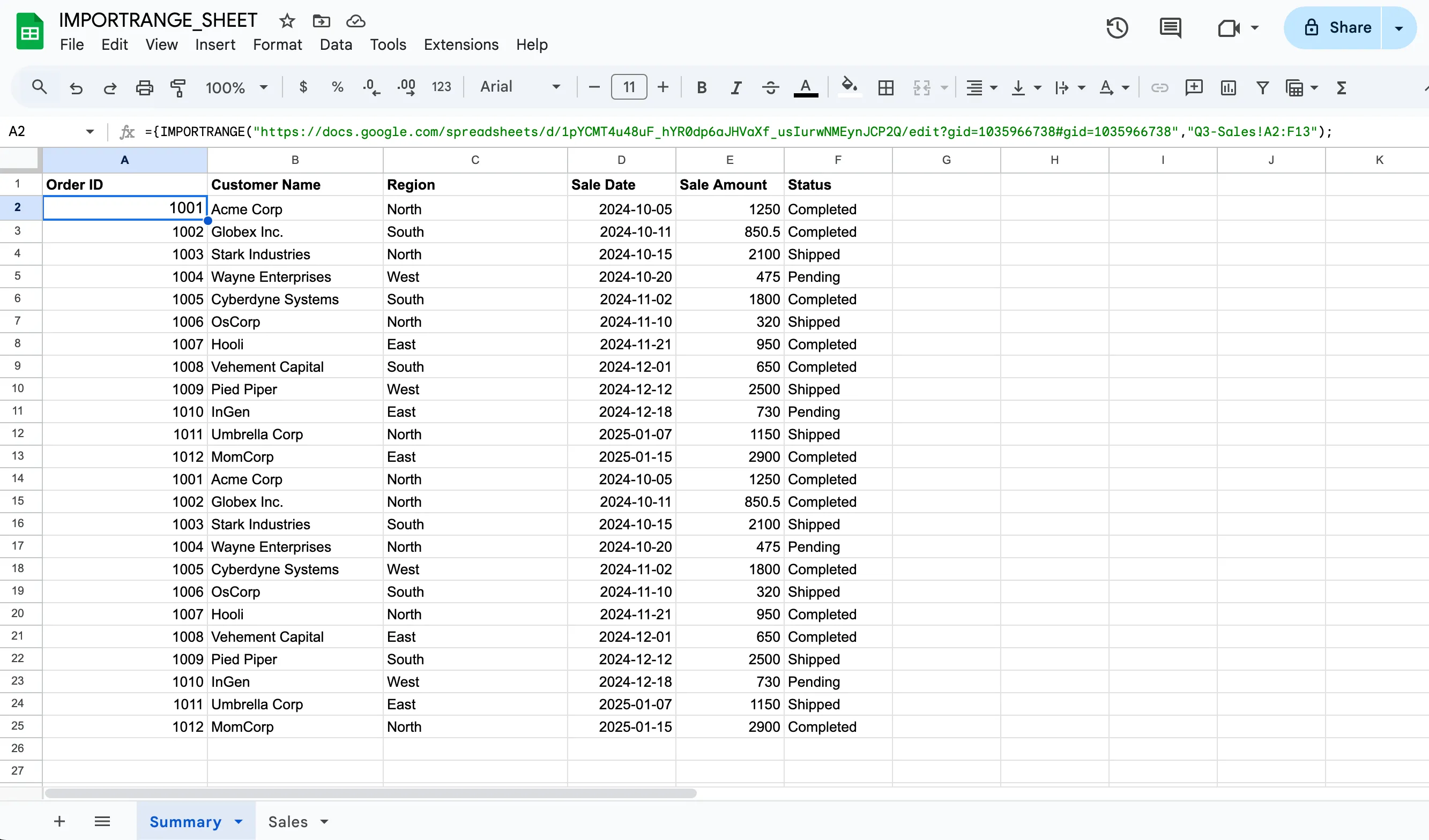
For instance, in case you have gross sales information cut up between “Q3-Gross sales” and “This autumn-Gross sales” sheets in your supply spreadsheet, you’ll be able to mix them vertically utilizing the system:

={IMPORTRANGE(sheet_URL,"Q3-Gross sales!A2:F13"); IMPORTRANGE(sheet_URL,"This autumn-Gross sales!A2:F13")}

This system first pulls the desired vary from “Q3-Gross sales.” The semicolon then tells it to append the info from “This autumn-Gross sales” straight beneath the Q3 information.

🔥 Please word that the variety of columns chosen in every IMPORTRANGE system are the identical else Google Sheets will return an error saying In ARRAY_LITERAL, an Array Literal was lacking values for a number of rows.

💡 We normally begin from cell A2 in each ranges. It is a widespread apply to keep away from importing the column headers twice, providing you with a clear, steady listing of information.

2.2. Horizontal Stacking (Place information side-by-side)

This technique is helpful when you have got information that’s unfold throughout a number of columns in several sheets. It permits you to mix information from totally different sheets right into a wider desk with extra columns.

To put ranges subsequent to one another horizontally, you employ the identical array syntax however separate the formulation with a comma contained in the curly braces {}. Right here you’ll be able to have totally different variety of rows in every vary however the variety of columns in every vary of the IMPORTRANGE system have to be the identical.

Let’s say you have got the client names within the Buyer sheet and their tackle particulars in an Handle sheet.

={IMPORTRANGE(sheet_URL,"Buyer!A2:B6"), IMPORTRANGE(sheet_URL,"Handle!A2:C6")}

The above system pulls buyer names from the primary vary and locations the tackle particulars from the second vary within the columns instantly to the suitable.

Be aware on Efficiency

You may completely use a number of IMPORTRANGE formulation in a single Google Sheet. Nonetheless, it’s vital to do not forget that every system creates a reside connection to an exterior file. You probably have dozens of those features in a single sheet, it may decelerate your calculations, because it always checks for updates in supply sheets.

For optimum efficiency, use one IMPORTRANGE system to convey your entire uncooked dataset into a brand new, devoted tab in your report. Then, use a number of QUERY or FILTER formulation in your dashboard that reference this native, imported information.

This manner you’ll be able to solely create one exterior connection, and all subsequent filtering is completed inside your sheet, which is considerably quicker.

Google Maps Formulation for Google Sheets

#3. Conditional Imports with the QUERY perform

Whereas IMPORTRANGE is a simple possibility for importing information into your sheet, its true potential is unlocked whenever you management precisely what information comes by means of. Importing a whole dataset is commonly pointless; you usually solely want particular rows – like stock from a sure warehouse, or gross sales for a selected interval.

That is the place the QUERY perform turns into your strongest ally. By wrapping your IMPORTRANGE in a QUERY, you’ll be able to transfer past easy importing and start pulling information based mostly on a selected situation(s). The syntax for the QUERY perform is as follows:

=QUERY(IMPORTRANGE("spreadsheet_url", "vary"), "Your Question Assertion")

The spreadsheet_url is the URL of the spreadsheet from the place information shall be imported. The vary tells Google Sheets precisely which sheet and which cells you wish to import. The Question Assertion is your filter (eg: the place Col3 = ‘Confirmed’).

How you can use QUERY perform – Examples

3.1: Get All Information for a Particular Area

Our supply Google Spreadsheet has a sheet named Gross sales that comprises the client identify, the area, sale quantity and different particulars that we wish to import into our vacation spot sheet. The IMPORTRANGE perform will assist however we solely wish to import the info for the North area.

=QUERY(IMPORTRANGE("URL", "Gross sales!A1:F13"), "SELECT * WHERE Col3 = 'North'")

• SELECT * implies that we wish to import all columns from the supply sheet.
• WHERE Col3 = ‘North’ is the filter. It tells the question to solely return rows the place the third column (Col3, which is Area) is the same as North. Be aware that the textual content values are case-sensitive and have to be in single quotes.

The QUERY perform doesn’t see the unique spreadsheet however the last information array that’s returned by the IMPORTRANGE perform. Due to this fact, it refers back to the columns of the ensuing array by their order: Col1 is the primary column of your imported vary, Col2 is the second, and so forth.

3.2: Mix A number of Circumstances (AND)

You want a report of all “Accomplished” gross sales within the “South” area. The AND key phrase helps you to chain a number of circumstances. The question will solely return rows that fulfill each the circumstances:

=QUERY(IMPORTRANGE("URL", "Gross sales!A1:F13"), "SELECT * WHERE Col3 = 'South' AND Col6 = 'Accomplished'")

3.3: Filter by a Listing of Potential Values (OR)

You wish to see all gross sales information from both the “East” or “West” areas mixed in a single listing. The OR key phrase returns rows that match both situation, permitting you to test for a number of doable values in the identical column.

=QUERY(IMPORTRANGE("URL", "Gross sales!A1:F13"), "SELECT * WHERE Col3 = 'East' OR Col3 = 'West'")

3.4: Filter by a Numerical Worth

It’s worthwhile to generate an inventory of all high-value gross sales the place the sale quantity is over $1,000. You should use customary comparability operators >, <, >=, <=, = for numbers. Discover that numbers and forex values are not positioned in quotes.

=QUERY(IMPORTRANGE("URL", "Gross sales!A1:F13"), "SELECT * WHERE Col5 > 1000")

3.5: Choose Particular Columns with Sorting

You need a clear report exhibiting simply the Buyer Title and Sale Quantity for high-value gross sales, with the most important gross sales showing first.

=QUERY(IMPORTRANGE("URL", "Sale!A1:F12"), "SELECT Col2, Col5 WHERE Col5 > 1000 ORDER BY Col5 DESC")

• SELECT Col2, Col5 specifies that we solely wish to import the “Buyer Title” and “Sale Quantity” columns.
• ORDER BY Col5 DESC kinds the outcomes based mostly on the “Sale Quantity” column (Col5) in descending order. Use ASC for ascending order.

3.6: Filter by a Date Vary

It’s worthwhile to see all gross sales that occurred within the fourth quarter of 2024 (from October 1st to December thirty first). When working with dates in QUERY, you should use the date key phrase adopted by the date in ‘YYYY-MM-DD’ format, enclosed in single quotes.

=QUERY(IMPORTRANGE("URL", "Gross sales!A1:F13"), "SELECT * WHERE Col4 >= date '2024-10-01' AND Col4 <= date '2024-12-31'")

3.7: Discover Partial Textual content Matches

You wish to discover all gross sales made to any firm with “Inc” in its identify. The comprises operator is ideal for locating a substring inside a textual content area.

=QUERY(IMPORTRANGE("URL", "Gross sales!A1:F12"), "SELECT * WHERE Col2 comprises 'Inc'")

It’s also possible to use begins with, ends with or matches operators to filter textual content values based mostly on common expressions.

3.8: Limiting the Variety of Outcomes

You wish to create a High 5 leaderboard exhibiting the most important gross sales. The LIMIT clause permits you to limit the variety of rows returned.

=QUERY(IMPORTRANGE("URL", "Gross sales!A1:F12"), "SELECT * ORDER by Col5 DESC LIMIT 5")

3.9: Aggregating Information to Create Summaries

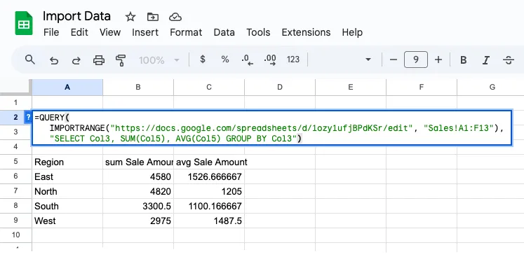
As a substitute of an extended listing of gross sales, you need a abstract desk exhibiting the overall gross sales worth for every area. The GROUP BY clause aggregates rows and allows you to carry out calculations on them with features like SUM(), COUNT(), and AVG().

=QUERY(IMPORTRANGE("URL", "Gross sales!A1:F12"), "SELECT Col3, SUM(Col5), AVG(Col5) GROUP BY Col3")

The GROUP BY Col3 clause scans the Area column and finds all of the distinctive values (North, South, East, West). It then creates a single output row for every area. The combination features SUM(Col5) and AVG(Col5) then calculate the overall and common gross sales quantity for all rows that belong to that area.

Different helpful combination features embody COUNT(), MAX(), and MIN().

3.10: Rename Column Titles in QUERY output

Google Sheets routinely names the columns within the output of a QUERY perform based mostly on the system used. For instance, in the event you use SELECT Col3, SUM(Col5) GROUP BY Col3, the output could have column titles like sum Sale Quantity that aren’t very descriptive. The LABEL clause helps you to rename these output headers for higher readability.

=QUERY(IMPORTRANGE("URL", "Gross sales!A1:F12"), "SELECT Col3, SUM(Col5) GROUP BY Col3 LABEL SUM(Col5) 'Whole Gross sales', Col3 'Gross sales Area'")

The syntax is LABEL column_to_rename new_column_name. You may chain a number of labels with a comma. This solely modifications your header in your output, it doesn’t have an effect on the unique supply information in any manner.

3.11: Formatting Date and Numbers

You may management how numbers and dates are displayed straight inside your question output utilizing the FORMAT clause. That is nice for making use of forex symbols or standardizing date codecs with out manually formatting your entire column.

=QUERY(IMPORTRANGE("URL", "Gross sales!A1:F12"), "SELECT Col3, SUM(Col5) GROUP BY Col3 LABEL SUM(Col5) 'Whole Gross sales' FORMAT SUM(Col5) '$#,##0.00'")

The sample '$#,##0.00' tells Sheets to show the quantity with a greenback signal, a comma for the 1000’s separator, and two decimal locations. That is purely visible, the underlying worth remains to be a quantity. You could possibly format a date with a sample like mmm d, yyyy to get Jul 15, 2025.

3.12: Transpose Information with PIVOT

You should use the PIVOT clause in your QUERY perform to rework your information from an inventory into a large, cross-tabulated abstract, just like a conventional Pivot Desk. That is significantly helpful whenever you wish to see how values in a single column (like gross sales quantities) are distributed throughout classes from one other column (like areas).

=QUERY(IMPORTRANGE("URL", "Gross sales!A1:F12"), "SELECT Col3, SUM(Col5) GROUP BY Col3 PIVOT Col6")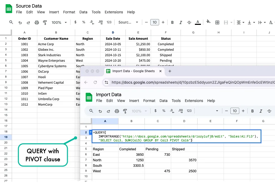

This question does three issues:

• GROUP BY Col3 creates a singular row for every area.
• SUM(Col5) decides what worth shall be calculated for the cells.
• PIVOT Col6 takes the distinctive values from the “Standing” column (Accomplished, Shipped, Pending) and turns them into their very own columns. The outcomes is a desk exhibiting the overall gross sales worth for every area, damaged down by standing.

3.13: Utilizing a Cell Reference as a Situation

You can also make your queries dynamic and interactive by constructing the question string to reference one other cell. That is the muse for creating dashboards that react to consumer enter.

To filter by textual content from a cell (e.g., cell G1 comprises the area identify), use this system:

=QUERY(IMPORTRANGE("URL", "Gross sales!A1:F12"), "SELECT * WHERE Col3 = '"&G1&"'")

Discover how we use the ampersand & operator to concatenate the worth from cell G1 into the question string. Textual content values should be enclosed in single quotes inside the QUERY string.

For those who have been filtering by a quantity from cell G1, the syntax can be easier:

=QUERY(IMPORTRANGE("URL", "Gross sales!A1:F12"), "SELECT * WHERE Col5 > " & G1)

3.14: Use QUERY with A number of Ranges

Whereas the QUERY perform solely takes a single information vary as its enter, you should use the curly braces {} syntax to create a single mixed vary from a number of sheets after which apply the QUERY perform to filter that mixed information. Right here is an instance:

=QUERY(
   {
      IMPORTRANGE("URL", "Q3-Gross sales!A1:F12"),
      IMPORTRANGE("URL", "This autumn-Gross sales!A1:F12")
   },
   "SELECT * WHERE Col6 = 'North'"
)

Right here’s how this system works step-by-step:

• Google Sheets evaluates the expressions contained in the curly braces first. This implies it executes each IMPORTRANGE features and combines their outcomes right into a single unified desk.
• The semicolon between the IMPORTRANGE features tells Sheets to stack the outcomes vertically – the second vary will seem straight beneath the primary vary.
• As soon as the info is mixed right into a single vertical desk, the QUERY perform processes this merged dataset as if it have been a single desk.

Vital: When stacking ranges this manner, every IMPORTRANGE should return the identical variety of columns.

#4. Import Information from the Identical Spreadsheet

Whereas IMPORTRANGE is important for pulling information from separate recordsdata, what in case your information resides in a unique tab inside the identical spreadsheet? For this situation, you don’t want the IMPORTRANGE perform however straight reference the cell within the supply sheet.

To reference a single cell from one other sheet, you merely sort =, adopted by the sheet identify, an exclamation mark, and the cell you wish to pull the info from.

=Gross sales!E14

To reference a spread of cells from one other tab, you employ the identical syntax as above however wrap it in curly braces {}. This instructs Google Sheet to output your entire array of information, not only a single worth.

={Gross sales!A1:D10}

A typical sample is to mix native cell referencing with the QUERY perform. This lets you hold your uncooked information in a single tab whereas creating a number of, filtered reviews in different tabs – all inside a single, quick loading spreadsheet.

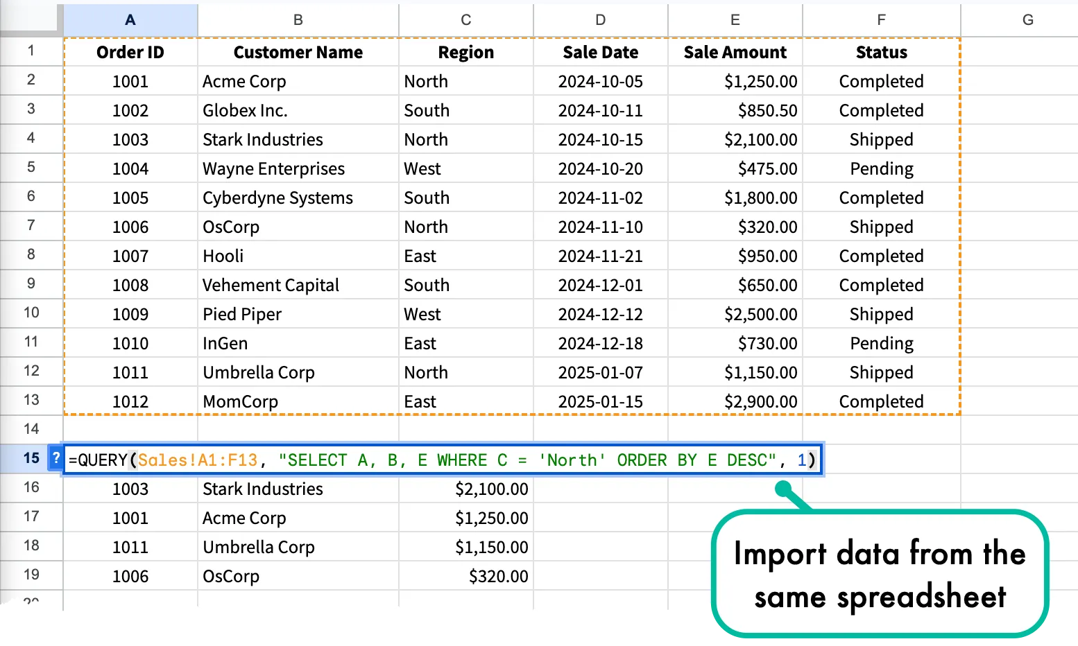
While you use QUERY on a spread from inside the spreadsheet, you’ll be able to straight use the precise column letters (A,B,C) in your QUERY assertion, as a substitute of utilizing the column numbers (Col1, Col2, Col3). It is because QUERY is referencing the native sheet straight and may see its construction.

=QUERY(Gross sales!A1:F12, "SELECT A, B, E WHERE C = 'North' ORDER BY E DESC")

The above QUERY perform pulls the info from the Gross sales sheet and filters it to solely embody the rows the place the Area column is the same as North. It then kinds the outcomes by the Sale Quantity column in descending order.

Importing Information – Which Technique to Use?

Whether or not your information lives in one other spreadsheet or in one other tab of the identical sheet, Google Sheets offers dependable and automatic methods to import information and in addition guaranteeing that your reviews and dashboards are at all times updated.

To summarize:

• If it is advisable to pull information from a totally totally different spreadsheet, your start line will at all times be the IMPORTRANGE perform.
• If it is advisable to filter, type or manipulate information, you need to wrap your IMPORTRANGE inside a QUERY perform.

Additionally see: Create Google Sheets Screenshots